Advance Filter

 

Filter by using advanced criteria

To open the Advanced Filter dialog box, click Data > Advanced.

	Example
	Salesperson = "Davolio" OR Salesperson = "Buchanan"
	Type = "Produce" AND Sales > 1000
	Type = "Produce" OR Salesperson = "Buchanan"
	(Sales > 6000 AND Sales < 6500 ) OR (Sales < 500)
	(Salesperson = "Davolio" AND Sales >3000) OR (Salesperson = "Buchanan" AND Sales > 1500)
	Salesperson = a name with 'u' as the second letter

Overview

The Advanced command works differently from the Filter command in several important ways.

• It displays the Advanced Filter dialog box instead of the AutoFilter menu.

• You type the advanced criteria in a separate criteria range on the worksheet and above the range of cells or table that you want to filter. Microsoft Office Excel uses the separate criteria range in the Advanced Filter dialog box as the source for the advanced criteria.

Sample data

The following sample data is used for all procedures in this article.

The data includes four blank rows above the list range that will be used as a criteria range (A1:C4) and a list range (A6:C10). The criteria range has column labels and includes at least one blank row between the criteria values and the list range.

To work with this data, select it in the following table, copy it, and then paste it in cell A1 of a new Excel worksheet.

Type	Salesperson	Sales
Type	Salesperson	Sales
Beverages	Suyama	$5122
Meat	Davolio	$450
produce	Buchanan	$6328
Produce	Davolio	$6544

Comparison operators

You can compare two values by using the following operators. When two values are compared by using these operators, the result is a logical value—either TRUE or FALSE.

Comparison operator	Meaning	Example
= (equal sign)	Equal to	A1=B1
> (greater than sign)	Greater than	A1>B1
< (less than sign)	Less than	A1<B1
>= (greater than or equal to sign)	Greater than or equal to	A1>=B1
<= (less than or equal to sign)	Less than or equal to	A1<=B1
<> (not equal to sign)	Not equal to	A1<>B1

Using the equal sign to type text or a value

Because the equal sign (=) is used to indicate a formula when you type text or a value in a cell, Excel evaluates what you type; however, this may cause unexpected filter results. To indicate an equality comparison operator for either text or a value, type the criteria as a string expression in the appropriate cell in the criteria range:

=''= entry ''

Where entry is the text or value you want to find. For example:

What you type in the cell	What Excel evaluates and displays
="=Davolio"	=Davolio
="=3000"	=3000

Considering case-sensitivity

When filtering text data, Excel doesn't distinguish between uppercase and lowercase characters. However, you can use a formula to perform a case-sensitive search. For an example, see the section Wildcard criteria.

Using pre-defined names

You can name a range Criteria, and the reference for the range will appear automatically in the Criteria range box. You can also define the name Database for the list range to be filtered and define the name Extract for the area where you want to paste the rows, and these ranges will appear automatically in the List range and Copy to boxes, respectively.

Creating criteria by using a formula

You can use a calculated value that is the result of a formula as your criterion. Remember the following important points:

• The formula must evaluate to TRUE or FALSE.

• Because you are using a formula, enter the formula as you normally would, and do not type the expression in the following way:

  =''= entry ''

• Do not use a column label for criteria labels; either keep the criteria labels blank or use a label that is not a column label in the list range (in the examples that follow, Calculated Average and Exact Match).

  If you use a column label in the formula instead of a relative cell reference or a range name, Excel displays an error value such as #NAME? or #VALUE! in the cell that contains the criterion. You can ignore this error because it does not affect how the list range is filtered.

• The formula that you use for criteria must use a relative reference to refer to the corresponding cell in the first row of data.

• All other references in the formula must be absolute references.

Multiple criteria, one column, any criteria true

Boolean logic:    (Salesperson = "Davolio" OR Salesperson = "Buchanan")

1. Insert at least three blank rows above the list range that can be used as a criteria range. The criteria range must have column labels. Make sure that there is at least one blank row between the criteria values and the list range.

2. To find rows that meet multiple criteria for one column, type the criteria directly below each other in separate rows of the criteria range. Using the example, enter:

   Type	Salesperson	Sales
   	="=Davolio"
   	="=Buchanan"

3. Click a cell in the list range. Using the example, click any cell in the range A6:C10.

4. On the Data tab, in the Sort & Filter group, click Advanced.

   

5. Do one of the following:

   • To filter the list range by hiding rows that don't match your criteria, click Filter the list, in-place.

   • To filter the list range by copying rows that match your criteria to another area of the worksheet, click Copy to another location, click in the Copy to box, and then click the upper-left corner of the area where you want to paste the rows.

     Tip    When you copy filtered rows to another location, you can specify which columns to include in the copy operation. Before filtering, copy the column labels for the columns that you want to the first row of the area where you plan to paste the filtered rows. When you filter, enter a reference to the copied column labels in the Copy to box. The copied rows will then include only the columns for which you copied the labels.

6. In the Criteria range box, enter the reference for the criteria range, including the criteria labels. Using the example, enter $A$1:$C$3.

   To move the Advanced Filter dialog box out of the way temporarily while you select the criteria range, click Collapse Dialog .

7. Using the example, the filtered result for the list range is:

   Type	Salesperson	Sales
   Meat	Davolio	$450
   produce	Buchanan	$6,328
   Produce	Davolio	$6,544

Multiple criteria, multiple columns, all criteria true

Boolean logic:    (Type = "Produce" AND Sales > 1000)

1. Insert at least three blank rows above the list range that can be used as a criteria range. The criteria range must have column labels. Make sure that there is at least one blank row between the criteria values and the list range.

2. To find rows that meet multiple criteria in multiple columns, type all the criteria in the same row of the criteria range. Using the example, enter:

   Type	Salesperson	Sales
   ="=Produce"		>1000

3. Click a cell in the list range. Using the example, click any cell in the range A6:C10.

4. On the Data tab, in the Sort & Filter group, click Advanced.

   

5. Do one of the following:

   • To filter the list range by hiding rows that don't match your criteria, click Filter the list, in-place.

   • To filter the list range by copying rows that match your criteria to another area of the worksheet, click Copy to another location, click in the Copy to box, and then click the upper-left corner of the area where you want to paste the rows.

     Tip    When you copy filtered rows to another location, you can specify which columns to include in the copy operation. Before filtering, copy the column labels for the columns that you want to the first row of the area where you plan to paste the filtered rows. When you filter, enter a reference to the copied column labels in the Copy to box. The copied rows will then include only the columns for which you copied the labels.

6. In the Criteria range box, enter the reference for the criteria range, including the criteria labels. Using the example, enter $A$1:$C$2.

   To move the Advanced Filter dialog box out of the way temporarily while you select the criteria range, click Collapse Dialog .

7. Using the example, the filtered result for the list range is:

   Type	Salesperson	Sales
   produce	Buchanan	$6,328
   Produce	Davolio	$6,544

Multiple criteria, multiple columns, any criteria true

Boolean logic:     (Type = "Produce" OR Salesperson = "Buchanan")

1. Insert at least three blank rows above the list range that can be used as a criteria range. The criteria range must have column labels. Make sure that there is at least one blank row between the criteria values and the list range.

2. To find rows that meet multiple criteria in multiple columns where any criteria can be true, type the criteria in the different columns and rows of the criteria range. Using the example, enter:

   Type	Salesperson	Sales
   ="=Produce"
   	="=Buchanan"

3. Click a cell in the list range. Using the example, click any cell in the list range A6:C10.

4. On the Data tab, in the Sort & Filter group, click Advanced.

   

5. Do one of the following:

   • To filter the list range by hiding rows that don't match your criteria, click Filter the list, in-place.

   • To filter the list range by copying rows that match your criteria to another area of the worksheet, click Copy to another location, click in the Copy to box, and then click the upper-left corner of the area where you want to paste the rows.

   Tip: When you copy filtered rows to another location, you can specify which columns to include in the copy operation. Before filtering, copy the column labels for the columns that you want to the first row of the area where you plan to paste the filtered rows. When you filter, enter a reference to the copied column labels in the Copy to box. The copied rows will then include only the columns for which you copied the labels.

6. In the Criteria range box, enter the reference for the criteria range, including the criteria labels. Using the example, enter $A$1:$B$3.

   To move the Advanced Filter dialog box out of the way temporarily while you select the criteria range, click Collapse Dialog .

7. Using the example, the filtered result for the list range is:

   Type	Salesperson	Sales
   produce	Buchanan	$6,328
   Produce	Davolio	$6,544

Multiple sets of criteria, one column in all sets

Boolean logic:     ( (Sales > 6000 AND Sales < 6500 ) OR (Sales < 500) )

1. Insert at least three blank rows above the list range that can be used as a criteria range. The criteria range must have column labels. Make sure that there is at least one blank row between the criteria values and the list range.

2. To find rows that meet multiple sets of criteria where each set includes criteria for one column, include multiple columns with the same column heading. Using the example, enter:

   Type	Salesperson	Sales	Sales
   		>6000	<6500
   		<500

3. Click a cell in the list range. Using the example, click any cell in the list range A6:C10.

4. On the Data tab, in the Sort & Filter group, click Advanced.

   

5. Do one of the following:

   • To filter the list range by hiding rows that don't match your criteria, click Filter the list, in-place.

   • To filter the list range by copying rows that match your criteria to another area of the worksheet, click Copy to another location, click in the Copy to box, and then click the upper-left corner of the area where you want to paste the rows.

     Tip: When you copy filtered rows to another location, you can specify which columns to include in the copy operation. Before filtering, copy the column labels for the columns that you want to the first row of the area where you plan to paste the filtered rows. When you filter, enter a reference to the copied column labels in the Copy to box. The copied rows will then include only the columns for which you copied the labels.

6. In the Criteria range box, enter the reference for the criteria range, including the criteria labels. Using the example, enter $A$1:$D$3.

   To move the Advanced Filter dialog box out of the way temporarily while you select the criteria range, click Collapse Dialog .

7. Using the example, the filtered result for the list range is:

   Type	Salesperson	Sales
   Meat	Davolio	$450
   produce	Buchanan	$6,328

Multiple sets of criteria, multiple columns in each set

Boolean logic:    ( (Salesperson = "Davolio" AND Sales >3000) OR (Salesperson = "Buchanan" AND Sales > 1500) )

1. Insert at least three blank rows above the list range that can be used as a criteria range. The criteria range must have column labels. Make sure that there is at least one blank row between the criteria values and the list range.

2. To find rows that meet multiple sets of criteria, where each set includes criteria for multiple columns, type each set of criteria in separate columns and rows. Using the example, enter:

   Type	Salesperson	Sales
   	="=Davolio"	>3000
   	="=Buchanan"	>1500

3. Click a cell in the list range. Using the example, click any cell in the list range A6:C10.

4. On the Data tab, in the Sort & Filter group, click Advanced.

   

5. Do one of the following:

   • To filter the list range by hiding rows that don't match your criteria, click Filter the list, in-place.

   • To filter the list range by copying rows that match your criteria to another area of the worksheet, click Copy to another location, click in the Copy to box, and then click the upper-left corner of the area where you want to paste the rows.

     Tip    When you copy filtered rows to another location, you can specify which columns to include in the copy operation. Before filtering, copy the column labels for the columns that you want to the first row of the area where you plan to paste the filtered rows. When you filter, enter a reference to the copied column labels in the Copy to box. The copied rows will then include only the columns for which you copied the labels.

6. In the Criteria range box, enter the reference for the criteria range, including the criteria labels. Using the example, enter $A$1:$C$3.To move the Advanced Filter dialog box out of the way temporarily while you select the criteria range, click Collapse Dialog .

7. Using the example, the filtered result for the list range would be:

   Type	Salesperson	Sales
   produce	Buchanan	$6,328
   Produce	Davolio	$6,544

Wildcard criteria

Boolean logic:    Salesperson = a name with 'u' as the second letter

1. To find text values that share some characters but not others, do one or more of the following:

   • Type one or more characters without an equal sign (=) to find rows with a text value in a column that begin with those characters. For example, if you type the text Dav as a criterion, Excel finds "Davolio," "David," and "Davis."

   • Use a wildcard character.

     Use	To find
     ? (question mark)	Any single character For example, sm?th finds "smith" and "smyth"
     * (asterisk)	Any number of characters For example, *east finds "Northeast" and "Southeast"
     ~ (tilde) followed by ?, *, or ~	A question mark, asterisk, or tilde For example, fy91~? finds "fy91?"

2. Insert at least three blank rows above the list range that can be used as a criteria range. The criteria range must have column labels. Make sure that there is at least one blank row between the criteria values and the list range.

3. In the rows below the column labels, type the criteria that you want to match. Using the example, enter:

   Type	Salesperson	Sales
   ="=Me*"
   	="=?u*"

4. Click a cell in the list range. Using the example, click any cell in the list range A6:C10.

5. On the Data tab, in the Sort & Filter group, click Advanced.

   

6. Do one of the following:

   • To filter the list range by hiding rows that don't match your criteria, click Filter the list, in-place

   • To filter the list range by copying rows that match your criteria to another area of the worksheet, click Copy to another location, click in the Copy to box, and then click the upper-left corner of the area where you want to paste the rows.

     Tip: When you copy filtered rows to another location, you can specify which columns to include in the copy operation. Before filtering, copy the column labels for the columns that you want to the first row of the area where you plan to paste the filtered rows. When you filter, enter a reference to the copied column labels in the Copy to box. The copied rows will then include only the columns for which you copied the labels.

7. In the Criteria range box, enter the reference for the criteria range, including the criteria labels. Using the example, enter $A$1:$B$3.

   To move the Advanced Filter dialog box out of the way temporarily while you select the criteria range, click Collapse Dialog  .

8. Using the example, the filtered result for the list range is:

   Type	Salesperson	Sales
   Beverages	Suyama	$5,122
   Meat	Davolio	$450
   produce	Buchanan	$6,328

Validation

Try it!

1. Select the cell(s) you want to create a rule for.

2. Select Data >Data Validation.

         

3. On the Settings tab, under Allow, select an option:

   • Whole Number - to restrict the cell to accept only whole numbers.

   • Decimal - to restrict the cell to accept only decimal numbers.

   • List - to pick data from the drop-down list.

   • Date - to restrict the cell to accept only date.

   • Time - to restrict the cell to accept only time.

   • Text Length - to restrict the length of the text.

   • Custom – for custom formula.

4.  Under Data, select a condition.

5. Set the other required values based on what you chose for Allow and Data.

6. Select the Input Message tab and customize a message users will see when entering data.

7. Select the Show input message when cell is selected checkbox to display the message when the user selects or hovers over the selected cell(s).

8. Select the Error Alert tab to customize the error message and to choose a Style.

9. Select OK.

   Now, if the user tries to enter a value that is not valid, an Error Alert appears with your customized message.

Download our examples

Download an example workbook with all data validation examples in this article

If you're creating a sheet that requires users to enter data, you might want to restrict entry to a certain range of dates or numbers, or make sure that only positive whole numbers are entered. Excel can restrict data entry to certain cells by using data validation, prompt users to enter valid data when a cell is selected, and display an error message when a user enters invalid data.

Which version are you using?



• Which version are you using?
• Newer versions
• Office 2011

Restrict data entry

1. Select the cells where you want to restrict data entry.

2. On the Data tab, click Data Validation > Data Validation.

   Note: If the validation command is unavailable, the sheet might be protected or the workbook might be shared. You cannot change data validation settings if your workbook is shared or your sheet is protected. For more information about workbook protection, see Protect a workbook.

3. In the Allow box, select the type of data you want to allow, and fill in the limiting criteria and values.

   Note: The boxes where you enter limiting values will be labeled based on the data and limiting criteria that you have chosen. For example, if you choose Date as your data type, you will be able to enter limiting values in minimum and maximum value boxes labeled Start Date and End Date.

Prompt users for valid entries

When users click in a cell that has data entry requirements, you can display a message that explains what data is valid.

1. Select the cells where you want to prompt users for valid data entries.

2. On the Data tab, click Data Validation > Data Validation.

   Note: If the validation command is unavailable, the sheet might be protected or the workbook might be shared. You cannot change data validation settings if your workbook is shared or your sheet is protected. For more information about workbook protection, see Protect a workbook.

3. On the Input Message tab, select the Show input message when cell is selected check box.

4. In the Title box, type a title for your message.

5. In the Input message box, type the message that you want to display.

Display an error message when invalid data is entered

If you have data restrictions in place and a user enters invalid data into a cell, you can display a message that explains the error.

1. Select the cells where you want to display your error message.

2. On the Data tab, click Data Validation > Data Validation.

   Note: If the validation command is unavailable, the sheet might be protected or the workbook might be shared. You cannot change data validation settings if your workbook is shared or your sheet is protected. For more information about workbook protection, see Protect a workbook.

3. On the Error Alert tab, in the Title box, type a title for your message.

4. In the Error message box, type the message that you want to display if invalid data is entered.

5. Do one of the following:

   To	On the Style pop-up menu, select
   Require users to fix the error before proceeding	Stop
   Warn users that data is invalid, and require them to select Yes or No to indicate if they want to continue	Warning
   Warn users that data is invalid, but allow them to proceed after dismissing the warning message	Important

Restrict data entry

1. Select the cells where you want to restrict data entry.

2. On the Data tab, under Tools, click Validate.

   

   Note: If the validation command is unavailable, the sheet might be protected or the workbook may be shared. You cannot change data validation settings if your workbook is shared or your sheet is protected. For more information about workbook protection, see Protect a workbook.

3. On the Allow pop-up menu, select the type of data you want to allow.

4. On the Data pop-up menu, select the type of limiting criteria that you want, and then enter limiting values.

   Note: The boxes where you enter limiting values will be labeled based on the data and limiting criteria that you have chosen. For example, if you choose Date as your data type, you will be able to enter limiting values in minimum and maximum value boxes labeled Start Date and End Date.

Prompt users for valid entries

When users click in a cell that has data entry requirements, you can display a message that explains what data is valid.

1. Select the cells where you want to prompt users for valid data entries.

2. On the Data tab, under Tools, click Validate.

   

   Note: If the validation command is unavailable, the sheet might be protected or the workbook may be shared. You cannot change data validation settings if your workbook is shared or your sheet is protected. For more information about workbook protection, see Protect a workbook.

3. On the Input Message tab, select the Show input message when cell is selected check box.

4. In the Title box, type a title for your message.

5. In the Input message box, type the message that you want to display.

Display an error message when invalid data is entered

If you have data restrictions in place and a user enters invalid data into a cell, you can display a message that explains the error.

1. Select the cells where you want to display your error message.

2. On the Data tab, under Tools, click Validate.

   

   Note: If the validation command is unavailable, the sheet might be protected or the workbook may be shared. You cannot change data validation settings if your workbook is shared or your sheet is protected. For more information about workbook protection, see Protect a workbook.

3. On the Error Alert tab, in the Title box, type a title for your message.

4. In the Error message box, type the message that you want to display if invalid data is entered.

5. Do one of the following:

   To	On the Style pop-up menu, select
   Require users to fix the error before proceeding	Stop
   Warn users that data is invalid, and require them to select Yes or No to indicate if they want to continue	Warning
   Warn users that data is invalid, but allow them to proceed after dismissing the warning message	Important

Add data validation to a cell or a range

Note: The first two steps in this section are for adding any type of data validation. Steps 3-7 are specifically for creating a drop-down list. 

1. Select one or more cells to validate.

2. On the Data tab, in the Data Tools group, click Data Validation.

3. On the Settings tab, in the Allow box, select List.

4. In the Source box, type your list values, separated by commas. For example, type Low,Average,High.

5. Make sure that the In-cell dropdown check box is selected. Otherwise, you won't be able to see the drop-down arrow next to the cell.

6. To specify how you want to handle blank (null) values, select or clear the Ignore blank check box.

7. Test the data validation to make sure that it is working correctly. Try entering both valid and invalid data in the cells to make sure that your settings are working as you intended and your messages are appearing when you expect.

Notes: 

• After you create your drop-down list, make sure it works the way you want. For example, you might want to check to see if the cell is wide enough to show all your entries.

• Remove data validation - Select the cell or cells that contain the validation you want to delete, then go to Data > Data Validation and in the data validation dialog press the Clear All button, then click OK.

Adding other types of data validation

The following table lists other types of data validation and shows you ways to add it to your worksheets.

To do this:	Follow these steps:
Restrict data entry to whole numbers within limits.	Follow steps 1-2 above. From the Allow list, select Whole number. In the Data box, select the type of restriction that you want. For example, to set upper and lower limits, select between. Enter the minimum, maximum, or specific value to allow. You can also enter a formula that returns a number value. For example, say you're validating data in cell F1. To set a minimum limit of deductions to two times the number of children in that cell, select greater than or equal to in the Data box and enter the formula, =2*F1, in the Minimum box.
Restrict data entry to a decimal number within limits.	Follow steps 1-2 above. In the Allow box, select Decimal. In the Data box, select the type of restriction that you want. For example, to set upper and lower limits, select between. Enter the minimum, maximum, or specific value to allow. You can also enter a formula that returns a number value. For example, to set a maximum limit for commissions and bonuses of 6% of a salesperson's salary in cell E1, select less than or equal to in the Data box and enter the formula, =E1*6%, in the Maximum box. Note: To let a user enter percentages, for example 20%, select Decimal in the Allow box, select the type of restriction that you want in the Data box, enter the minimum, maximum, or specific value as a decimal, for example .2, and then display the data validation cell as a percentage by selecting the cell and clicking Percent Style in the Number group on the Home tab.
Restrict data entry to a date within range of dates.	Follow steps 1-2 above. In the Allow box, select Date. In the Data box, select the type of restriction that you want. For example, to allow dates after a certain day, select greater than. Enter the start, end, or specific date to allow. You can also enter a formula that returns a date. For example, to set a time frame between today's date and 3 days from today's date, select between in the Data box, enter =TODAY() in the Start date box, and enter =TODAY()+3 in the End date box.
Restrict data entry to a time within a time frame.	Follow steps 1-2 above. In the Allow box, select Time. In the Data box, select the type of restriction that you want. For example, to allow times before a certain time of day, select less than. Enter the start, end, or specific time to allow. If you want to enter specific times, use the hh:mm time format. For example, say you have cell E2 set up with a start time (8:00 AM), and cell F2 with an end time (5:00 PM), and you want to limit meeting times between those times then select between in the Data box, enter =E2 in the Start time box, and then enter =F2 in the End time box.
Restrict data entry to text of a specified length.	Follow steps 1-2 above. In the Allow box, select Text Length. In the Data box, select the type of restriction that you want. For example, to allow up to a certain number of characters, select less than or equal to. In this case we want to limit entry to 25 characters, so select less than or equal to in the Data box and enter 25 in the Maximum box.
Calculate what is allowed based on the content of another cell.	Follow steps 1-2 above. In the Allow box, select the type of data that you want. In the Data box, select the type of restriction that you want. In the box or boxes below the Data box, click the cell that you want to use to specify what is allowed. For example, to allow entries for an account only if the result won't go over the budget in cell E1, select Allow >Whole number, Data, less than or equal to, and Maximum >= =E1.

Examples of formulas in data validation

Notes: 

• The following examples use the Custom option where you write formulas to set your conditions. You don't need to worry about whatever the Data box shows, as that's disabled with the Custom option.

• The screen shots in this article were taken in Excel 2016; but the functionality is the same in Excel for the web.

To make sure that	Enter this formula
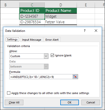
The cell that contains a product ID (C2) always begins with the standard prefix of "ID-" and is at least 10 (greater than 9) characters long.	=AND(LEFT(C2,3)="ID-",LEN(C2)>9)
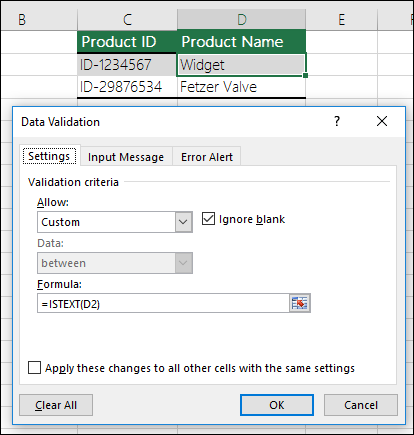
The cell that contains a product name (D2) only contains text.	=ISTEXT(D2)
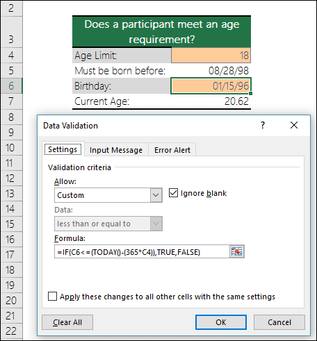
The cell that contains someone's birthday (B6) has to be greater than the number of years set in cell B4.	=IF(B6<=(TODAY()-(365*B4)),TRUE,FALSE)
All the data in the cell range A2:A10 contains unique values.	=COUNTIF($A$2:$A$10,A2)=1 Note: You must enter the data validation formula for cell A2 first, then copy A2 to A3:A10 so that the second argument to the COUNTIF will match the current cell. That is the A2)=1 portion will change to A3)=1, A4)=1 and so on. For more information
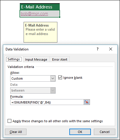
Ensure that an e-mail address entry in cell B4 contains the @ symbol.	=ISNUMBER(FIND("@",B4))

Part -1 Cell fixing in excel----(Nobody tells you about cell fixing)

I think you need to learn to fix cells before applying any formula. Because without fixing you cannot put any formula in the cell. This is very important term of Excel.

Let's know about Excel cell fixing-- The basis of Excel fixing is that if we fix the cell, the cell reference cannot move. 
We specify the following conditions of cell fixing.

(i) "$" (operator)- :  We always fix the cell using the $ dollar       operator

Please refer to the above picture carefully. We want to put 1 value in columns A3, A4, A5, A6, while we put 1 in columns B $ 3 using "$" dollar operator. Now we drag columns A3 to A6, we see that  A6 columns till get 1 value. 1 value comes because we used cell fix using $ operator.

Please refer to the above picture carefully. We want to put 1 value in columns A3, A4, A5, A6, while we put 1 in columns B3 Without using "$" dollar operator. Now we drag columns A3 to A6, we see that  A3 get 1 value. Rest Columns gets 0 Value Because B3 = 1 only while we drag A3 till A6 ,B3 reflecting 0, B4 reflecting 0,B5 reflecting 0 and B6 also reflecting 0 because we not use "$" Operator means we don't fix the cell.

The conclusion is that if we use "$" to fix the cell, the cell value does not change, but we do not use "$", the cell value changes. As stated in the example above

In the next post we will give another example with formula



To be Continued